High Jump

• Click on File → Open…, and open Tutorials/Tutorial 2a - High Jump.scone

In the editor, you'll see a section called 'Controller', with the following code:

# Controller for the Model
FeedForwardController {
	symmetric = 1
 
	# Function for feed-forward pattern
	PieceWiseConstant {
		control_points = 2
		control_point_y = 0.3~0.01<0,1> # Initial y value of control points
		control_point_dt = 0.2~0.01<0,1> # initial delta time between control points
	}
}

The FeedForwardController is the type of controller, and the Function defines the type of function. In this case, we define a PieceWiseConstantFunction function with two control points, and a variable time between control points. The values after control_point_y and control_point_dt define parameters to be optimized, and have the following format:

mean~standard deviation<minimum, maximum>

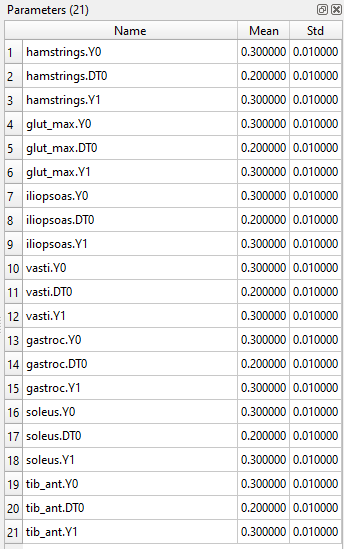
The actual parameters that are used in this scenario are shown in the Parameters Window (see picture on the right-hand side), which can be activated by Windows → Parameters. Here you will see the setpoints Y1 and Y2 for each muscle, as well as the time delta DT0 between the setpoints.

• To start the optimization, click on Scenario → Optimize Scenario

If you do not wish to optimize a parameter, for instance if you wish to use a piece-wise function with a fixed time interval of 0.1 seconds, simply change control_point_dt to:

control_point_dt = 0.1 # this parameter is no longer optimized

Alternatively, you can change the initial mean and standard deviation for each of the parameters.

Instead of using a PieceWiseConstantFunction function, it is also possible to use a PieceWiseLinearFunction function or a Polynomial, simply by changing the type of the function.

To use a polynomial to define the muscle excitation signal for each muscle, change the code into the following (see also Tutorials/Tutorial 2b - High Jump Polynomial.scone):

# Controller for the Model
FeedForwardController {
	symmetric = 1
 
	# 2nd degree polynomial ax^2 + bx + c
	Polynomial {
		degree = 2
		coefficient0 = 0.3~0.01<0,1> # initial value for c
		coefficient1 = 0~0.1<-10,10> # initial value for b
		coefficient2 = 0~0.1<-10,10> # initial value for a
	}
}

You can see in the Parameters window that the name of the parameters has changed – these now represent the coefficients of the polynomial function that describes the excitation curve for each muscle.

If you have run the optimization for a while, you will notice that the model has a tendency to lean backwards during the jump. The reason for this is that our optimization objective only cares about how high it jumps, not about the pose of its upper body.

The objective function is defined by the Objective and Measure tags. The objective type is a SimulationObjective, which is used for objective functions that are the result of a simulation. Inside the Objective you'll find the Measure that defines the fitness function of the objective.

By default, JumpMeasure measures the maximum height of the Center of Mass (COM) of the model. We can add an additional term to also take into account the orientation of the upper body (see also Tutorial 2c - Straight Pose Jump.scone):

# Composite measure for straight pose jumping
CompositeMeasure {
 
	# Fitness measure for jumping
	JumpMeasure {
		termination_height = 0.75
		prepare_time = 0.2
	}
 
	# Penalize backwards leaning pose
	DofMeasure {
		dof = pelvis_tilt
		position { min = -45 max = 0 abs_penalty = -10 }
	}
}

We changed the measure type to CompositeMeasure, and combine our JumpMeasure with an additional DofMeasure. The DofMeasure adds a penalty when a specific Degree of Freedom (DOF) is outside a specific range. In this case, we define the valid range to be between -45 and 0 degrees, and apply a fitness value of -10 per degree at which the pelvis_tilt is outside this range.

After clicking on one of the results, analyze the activation patterns in the Analysis tool, to find out what jumping strategies are found by the optimizer.